Predicting atomic forces with equivariant graph neural networks
To run a molecular dynamics simulation, we need to know the force on every atom at each time step. We can compute the forces if we know the potential energy function \(E\); the force on atom \(i\) is simply the negative gradient of the energy with respect to that atom’s position:
\[\mathbf{F}_i = -\nabla_{\mathbf{r}_i} E(\mathbf{r}_1, \ldots, \mathbf{r}_N).\]Unfortunately, correctly evaluating the potential energy for a given molecule requires expensive quantum mechanical calculations. Machine learning offers an attractive alternative: we can train a model \(\Phi_{\theta}\) on a dataset of molecular configurations with pre-computed ground truth forces and the use the trained model to predict forces for arbitrary configurations,
\[\left\{\mathbf{F}_1, \ldots, \mathbf{F}_N\right\} \approx \Phi_{\theta}(\mathbf{r}_1, \ldots, \mathbf{r}_N).\]In this post, I’ll discuss how to do this using E(n) equivariant graph neural networks (EGNNs), which are particularly well-suited for this task because they respect certain symmetries by construction (e.g., rotational symmetry: if we rotate a molecule, we want the predicted forces to rotate accordingly).
The data
The MD17 dataset contains ab-initio molecular dynamics trajectories for small organic molecules. Each configuration provides atomic positions, atomic numbers, and ground-truth forces computed via DFT. We’ll train on aspirin (21 atoms per configuration). Specifically, we’ll take 1000 configurations from the full trajectory and use 800 for training, 100 for validation, and 100 for testing.
We represent each configuration as a graph where nodes are atoms and edges connect atoms within a 5 Å cutoff. Each node carries both a 3D position vector and a one-hot encoding of the atom type:
from torch_geometric.datasets import MD17
from torch_geometric.transforms import RadiusGraph

dataset = MD17(root='./data', name='aspirin', transform=RadiusGraph(r=5.0, loop=False))

def create_node_features(atomic_numbers, max_atomic_num):
    """One-hot encode atomic numbers as node features."""
    x = torch.zeros(atomic_numbers.size(0), max_atomic_num, dtype=torch.float)
    x.scatter_(1, atomic_numbers.unsqueeze(1).long(), 1)
    return x
We can use py3Dmol to visualize the trajectory for the aspirin molecule:
3Dmol.js failed to load for some reason. Please check your browser console for error messages.
Our task is to predict \(3N\) force components (one 3D vector per atom). The visualization below shows a sample configuration in which the ground-truth force vectors are displayed as red arrows:
3Dmol.js failed to load for some reason. Please check your browser console for error messages.
The animation below shows the full graph (that is, the atoms along with the edges added by the RadiusGraph transform).

EGNN equations
Each EGNN layer updates both node features \(h_i\) and coordinates \(\mathbf{r}_i\) through message passing. For connected atoms \(i\) and \(j\):
Edge messages combine node features with squared distances (invariant to rotation):
\[m_{ij} = \phi_e(h_i, h_j, \|\mathbf{r}_i - \mathbf{r}_j\|^2)\]Node updates aggregate messages and apply a residual connection:
\[h_i^{l+1} = h_i^l + \phi_h\left(h_i^l, \sum_{j \in \mathcal{N}(i)} m_{ij}\right)\]Coordinate updates use scalar-weighted coordinate differences (equivariant):
\[\mathbf{r}_i^{l+1} = \mathbf{r}_i^l + \sum_{j \in \mathcal{N}(i)} \phi_x(m_{ij}) \cdot (\mathbf{r}_i - \mathbf{r}_j)\]Force prediction scales the total coordinate displacement by an invariant scalar:
\[\mathbf{F}_i = \phi_v(h_i^{\text{final}}) \cdot (\mathbf{r}_i^{\text{final}} - \mathbf{r}_i^{\text{initial}})\]All \(\phi\) functions are MLPs. The architecture maintains equivariance because coordinate updates depend only on coordinate differences—rotating the input rotates the output forces accordingly.
Training Procedure
We train the EGNN to minimize the mean squared error between predicted and ground truth forces:
\[\mathcal{L} = \frac{1}{N} \sum_{i=1}^{N} ||\mathbf{F}_i^{\text{pred}} - \mathbf{F}_i^{\text{true}}||^2\]where \(N\) is the number of atoms in the batch, and \(\mathbf{F}_i^{\text{pred}}\) and \(\mathbf{F}_i^{\text{true}}\) are the predicted and ground truth force vectors for atom \(i\).
Before training, we normalize forces to zero mean and unit variance using training set statistics to improve training stability.
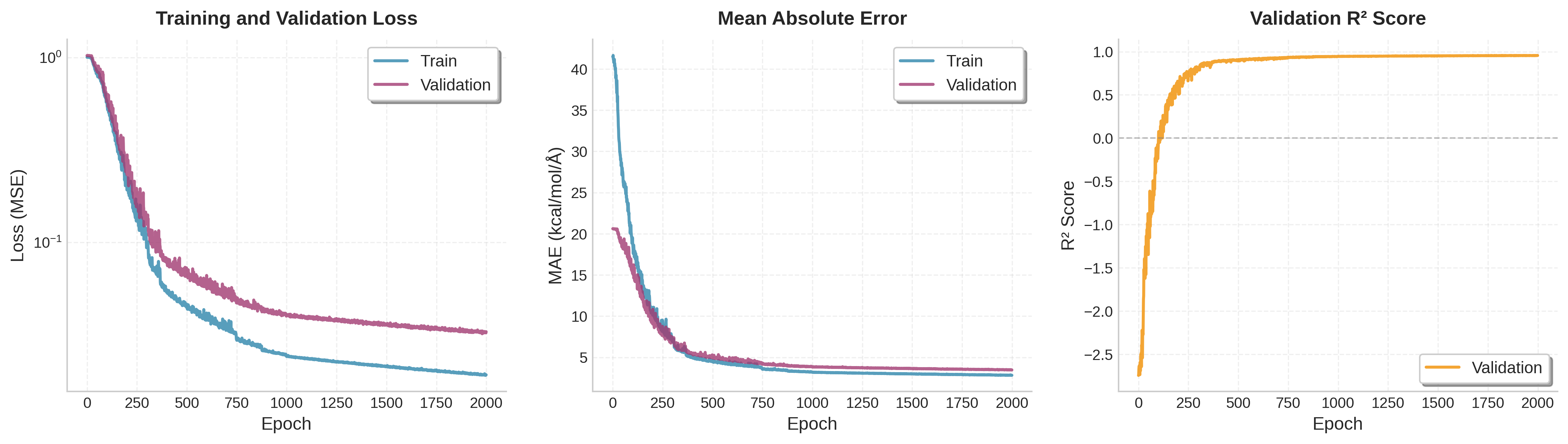
The training curves show steady convergence as the model learns to predict forces accurately: